


Pingouin is an open-source statistical package written in Python 3 and based mostly on Pandas and NumPy. Some of its main features are listed below. For a full list of available functions, please refer to the API documentation.
ANOVAs: N-ways, repeated measures, mixed, ancova
Pairwise post-hocs tests (parametric and non-parametric) and pairwise correlations
Robust, partial, distance and repeated measures correlations
Linear/logistic regression and mediation analysis
Bayes Factors
Multivariate tests
Reliability and consistency
Effect sizes and power analysis
Parametric/bootstrapped confidence intervals around an effect size or a correlation coefficient
Circular statistics
Chi-squared tests
Plotting: Bland-Altman plot, Q-Q plot, paired plot, robust correlation…
Pingouin is designed for users who want simple yet exhaustive stats functions.
For example, the ttest_ind function of SciPy returns only the T-value and the p-value. By contrast,
the ttest function of Pingouin returns the T-value, the p-value, the degrees of freedom, the effect size (Cohen’s d), the 95% confidence intervals of the difference in means, the statistical power and the Bayes Factor (BF10) of the test.
Installation#
Pingouin is a Python 3 package and is currently tested for Python 3.8-3.11.
The main dependencies of Pingouin are :
In addition, some functions require :
Pingouin can be easily installed using pip
pip install pingouin
or conda
conda install -c conda-forge pingouin
Pingouin is under heavy development and it is likely that bugs/mistakes will be discovered in future releases. Please always make sure that you are using the latest version of Pingouin (new releases are frequent). Whenever a new release is out there, you can upgrade your version by typing the following line in a terminal window:
pip install --upgrade pingouin
Quick start#
If you have questions, please ask them in GitHub Discussions.
If you want to report a bug, please open an issue on the GitHub repository.
If you want to see Pingouin in action, please click on the link below and navigate to the notebooks/ folder to open a collection of interactive Jupyter notebooks.

10 minutes to Pingouin#
1. T-test#
import numpy as np
import pingouin as pg

np.random.seed(123)
mean, cov, n = [4, 5], [(1, .6), (.6, 1)], 30
x, y = np.random.multivariate_normal(mean, cov, n).T

# T-test
pg.ttest(x, y)
T |
dof |
alternative |
p-val |
CI95% |
cohen-d |
BF10 |
power |
|---|---|---|---|---|---|---|---|
-3.401 |
58 |
two-sided |
0.001 |
[-1.68 -0.43] |
0.878 |
26.155 |
0.917 |
2. Pearson’s correlation#
pg.corr(x, y)
n |
r |
CI95% |
p-val |
BF10 |
power |
|---|---|---|---|---|---|
30 |
0.595 |
[0.3 0.79] |
0.001 |
69.723 |
0.950 |
3. Robust correlation#
# Introduce an outlier
x[5] = 18
# Use the robust biweight midcorrelation
pg.corr(x, y, method="bicor")
n |
r |
CI95% |
p-val |
power |
|---|---|---|---|---|
30 |
0.576 |
[0.27 0.78] |
0.001 |
0.933 |
4. Test the normality of the data#
The pingouin.normality() function works with lists, arrays, or pandas DataFrame in wide or long-format.
print(pg.normality(x))                                    # Univariate normality
print(pg.multivariate_normality(np.column_stack((x, y)))) # Multivariate normality
W |
pval |
normal |
|---|---|---|
0.615 |
0.000 |
False |
(False, 0.00018)
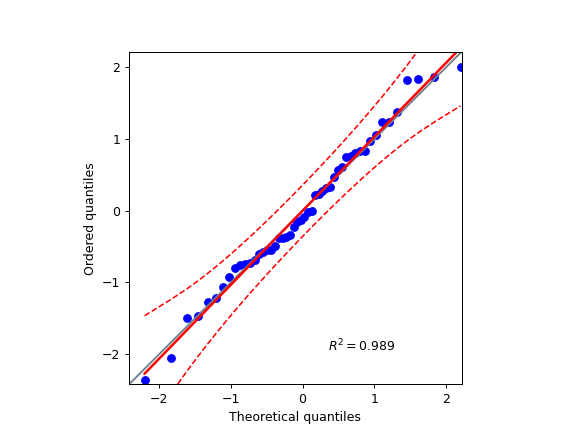
5. Q-Q plot#
import numpy as np
import pingouin as pg
np.random.seed(123)
x = np.random.normal(size=50)
ax = pg.qqplot(x, dist='norm')
6. One-way ANOVA using a pandas DataFrame#
# Read an example dataset
df = pg.read_dataset('mixed_anova')

# Run the ANOVA
aov = pg.anova(data=df, dv='Scores', between='Group', detailed=True)
print(aov)
Source |
SS |
DF |
MS |
F |
p-unc |
np2 |
|---|---|---|---|---|---|---|
Group |
5.460 |
1 |
5.460 |
5.244 |
0.023 |
0.029 |
Within |
185.343 |
178 |
1.041 |
nan |
nan |
nan |
7. Repeated measures ANOVA#
pg.rm_anova(data=df, dv='Scores', within='Time', subject='Subject', detailed=True)
Source |
SS |
DF |
MS |
F |
p-unc |
ng2 |
eps |
|---|---|---|---|---|---|---|---|
Time |
7.628 |
2 |
3.814 |
3.913 |
0.023 |
0.04 |
0.999 |
Error |
115.027 |
118 |
0.975 |
nan |
nan |
nan |
nan |
8. Post-hoc tests corrected for multiple-comparisons#
# FDR-corrected post hocs with Hedges'g effect size
posthoc = pg.pairwise_tests(data=df, dv='Scores', within='Time', subject='Subject',
                             parametric=True, padjust='fdr_bh', effsize='hedges')

# Pretty printing of table
pg.print_table(posthoc, floatfmt='.3f')
Contrast |
A |
B |
Paired |
Parametric |
T |
dof |
alternative |
p-unc |
p-corr |
p-adjust |
BF10 |
hedges |
|---|---|---|---|---|---|---|---|---|---|---|---|---|
Time |
August |
January |
True |
True |
-1.740 |
59.000 |
two-sided |
0.087 |
0.131 |
fdr_bh |
0.582 |
-0.328 |
Time |
August |
June |
True |
True |
-2.743 |
59.000 |
two-sided |
0.008 |
0.024 |
fdr_bh |
4.232 |
-0.483 |
Time |
January |
June |
True |
True |
-1.024 |
59.000 |
two-sided |
0.310 |
0.310 |
fdr_bh |
0.232 |
-0.170 |
9. Two-way mixed ANOVA#
# Compute the two-way mixed ANOVA and export to a .csv file
aov = pg.mixed_anova(data=df, dv='Scores', between='Group', within='Time',
                     subject='Subject', correction=False, effsize="np2")
pg.print_table(aov)
Source |
SS |
DF1 |
DF2 |
MS |
F |
p-unc |
np2 |
eps |
|---|---|---|---|---|---|---|---|---|
Group |
5.460 |
1 |
58 |
5.460 |
5.052 |
0.028 |
0.080 |
nan |
Time |
7.628 |
2 |
116 |
3.814 |
4.027 |
0.020 |
0.065 |
0.999 |
Interaction |
5.167 |
2 |
116 |
2.584 |
2.728 |
0.070 |
0.045 |
nan |
10. Pairwise correlations between columns of a dataframe#
import pandas as pd
np.random.seed(123)
z = np.random.normal(5, 1, 30)
data = pd.DataFrame({'X': x, 'Y': y, 'Z': z})
pg.pairwise_corr(data, columns=['X', 'Y', 'Z'], method='pearson')
X |
Y |
method |
alternative |
n |
r |
CI95% |
p-unc |
BF10 |
power |
|---|---|---|---|---|---|---|---|---|---|
X |
Y |
pearson |
two-sided |
30 |
0.366 |
[0.01 0.64] |
0.047 |
1.500 |
0.525 |
X |
Z |
pearson |
two-sided |
30 |
0.251 |
[-0.12 0.56] |
0.181 |
0.534 |
0.272 |
Y |
Z |
pearson |
two-sided |
30 |
0.020 |
[-0.34 0.38] |
0.916 |
0.228 |
0.051 |
11. Pairwise T-test between columns of a dataframe#
data.ptests(paired=True, stars=False)
X |
Y |
Z |
|
|---|---|---|---|
X |
0.226 |
0.165 |
|
Y |
-1.238 |
0.658 |
|
Z |
-1.424 |
-0.447 |
12. Multiple linear regression#
pg.linear_regression(data[['X', 'Z']], data['Y'])
names |
coef |
se |
T |
pval |
r2 |
adj_r2 |
CI[2.5%] |
CI[97.5%] |
|---|---|---|---|---|---|---|---|---|
Intercept |
4.650 |
0.841 |
5.530 |
0.000 |
0.139 |
0.076 |
2.925 |
6.376 |
X |
0.143 |
0.068 |
2.089 |
0.046 |
0.139 |
0.076 |
0.003 |
0.283 |
Z |
-0.069 |
0.167 |
-0.416 |
0.681 |
0.139 |
0.076 |
-0.412 |
0.273 |
13. Mediation analysis#
pg.mediation_analysis(data=data, x='X', m='Z', y='Y', seed=42, n_boot=1000)
path |
coef |
se |
pval |
CI[2.5%] |
CI[97.5%] |
sig |
|---|---|---|---|---|---|---|
Z ~ X |
0.103 |
0.075 |
0.181 |
-0.051 |
0.256 |
No |
Y ~ Z |
0.018 |
0.171 |
0.916 |
-0.332 |
0.369 |
No |
Total |
0.136 |
0.065 |
0.047 |
0.002 |
0.269 |
Yes |
Direct |
0.143 |
0.068 |
0.046 |
0.003 |
0.283 |
Yes |
Indirect |
-0.007 |
0.025 |
0.898 |
-0.069 |
0.029 |
No |
14. Contingency analysis#
data = pg.read_dataset('chi2_independence')
expected, observed, stats = pg.chi2_independence(data, x='sex', y='target')
stats
test |
lambda |
chi2 |
dof |
p |
cramer |
power |
|---|---|---|---|---|---|---|
pearson |
1.000 |
22.717 |
1.000 |
0.000 |
0.274 |
0.997 |
cressie-read |
0.667 |
22.931 |
1.000 |
0.000 |
0.275 |
0.998 |
log-likelihood |
0.000 |
23.557 |
1.000 |
0.000 |
0.279 |
0.998 |
freeman-tukey |
-0.500 |
24.220 |
1.000 |
0.000 |
0.283 |
0.998 |
mod-log-likelihood |
-1.000 |
25.071 |
1.000 |
0.000 |
0.288 |
0.999 |
neyman |
-2.000 |
27.458 |
1.000 |
0.000 |
0.301 |
0.999 |
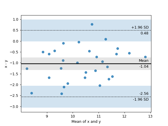
15. Bland-Altman plot#
import numpy as np
import pingouin as pg
np.random.seed(123)
mean, cov = [10, 11], [[1, 0.8], [0.8, 1]]
x, y = np.random.multivariate_normal(mean, cov, 30).T
ax = pg.plot_blandaltman(x, y)
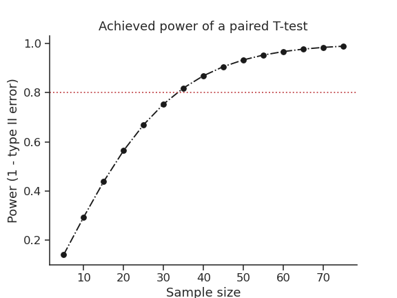
16. Plot achieved power of a paired T-test#
Plot the curve of achieved power given the effect size (Cohen d) and the sample size of a paired T-test.
import matplotlib.pyplot as plt
import seaborn as sns
import pingouin as pg
import numpy as np
sns.set(style='ticks', context='notebook', font_scale=1.2)
d = 0.5  # Fixed effect size
n = np.arange(5, 80, 5)  # Incrementing sample size
# Compute the achieved power
pwr = pg.power_ttest(d=d, n=n, contrast='paired')
# Start the plot
plt.plot(n, pwr, 'ko-.')
plt.axhline(0.8, color='r', ls=':')
plt.xlabel('Sample size')
plt.ylabel('Power (1 - type II error)')
plt.title('Achieved power of a paired T-test')
sns.despine()
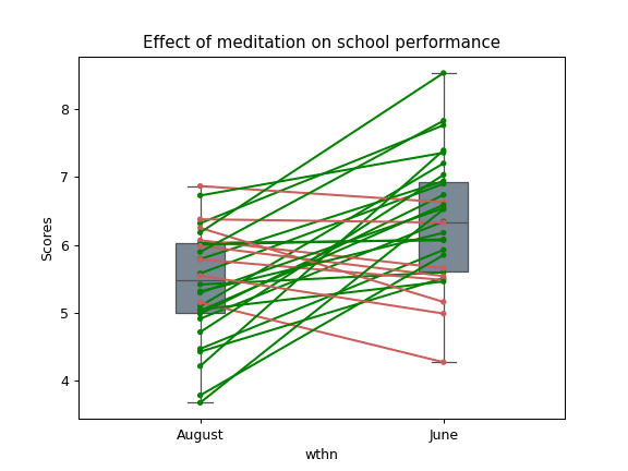
17. Paired plot#
import pingouin as pg
import numpy as np
df = pg.read_dataset('mixed_anova').query("Group == 'Meditation' and Time != 'January'")
ax = pg.plot_paired(data=df, dv='Scores', within='Time', subject='Subject')
ax.set_title("Effect of meditation on school performance")
Integration with Pandas#
Several functions of Pingouin can be used directly as pandas.DataFrame methods. Try for yourself with the code below:
import pingouin as pg

# Example 1 | ANOVA
df = pg.read_dataset('mixed_anova')
df.anova(dv='Scores', between='Group', detailed=True)

# Example 2 | Pairwise correlations
data = pg.read_dataset('mediation')
data.pairwise_corr(columns=['X', 'M', 'Y'], covar=['Mbin'])

# Example 3 | Partial correlation matrix
data.pcorr()
The functions that are currently supported as pandas method are:
Development#
Pingouin was created and is maintained by Raphael Vallat, a postdoctoral researcher at UC Berkeley, mostly during his spare time. Contributions are more than welcome so feel free to contact me, open an issue or submit a pull request!
To see the code or report a bug, please visit the GitHub repository.
This program is provided with NO WARRANTY OF ANY KIND. Pingouin is still under heavy development and there are likely hidden bugs. Always double check the results with another statistical software.
Contributors
Nicolas Legrand
Acknowledgement#
Several functions of Pingouin were inspired from R or Matlab toolboxes, including: